


Introduction
ImageJ will celebrate its tenth anniversary in September of this year. These past 10 years have seen the Java-based open-source software mature into an invaluable laboratory tool. In addition to its impressive functionality, this cutting-edge image-processing tool has an indispensable support community of enthusiasts on the ImageJ mailing list.
Wayne Rasband is the core author of ImageJ; after developing the Macintosh-based National Institutes of Health (NIH) Image for 10 years, he made the brave decision of starting afresh with ImageJ using the Java programming language. By shifting to Java, Rasband liberated the software from an individual operating system. To run ImageJ, a given system needs only the operating system-specific Java runtime environment. Java runtime environments (JRE) are freely available, either from Sun or bundled with platform-specific installations of ImageJ (rsb.info.nih.gov/ij). With JRE available for most operating systems, ImageJ is platform-independent, running on Macintosh, Windows, Linux, and even a PDA operating system. The new 64-bit operating systems and their JRE have happily broken the long-held 1.7 Gb memory limit for Java applications. One of the downsides of the Java heritage is an interface that may feel a little unfamiliar. However, a few steps into ImageJ, and this minor inconvenience is forgotten.
While Rasband is the author of the core program, an extensive group of additional developers has written and made available a growing arsenal of short add-on programs to provide additional functionality to the core program. These additional files are either written in Java (the plugins) or in ImageJ's macro programming language (macros). Once saved to the ImageJ plugins folder, these functions are loaded on start-up and can be accessed via menu commands like any other core function.
400+ Plugins
Freely available for individual download, the 400+ plugins contribute to the success of ImageJ, but can also be overwhelming by their sheer magnitude. Where to start? One at a time?
The long list of plugins reflects ImageJ's usage throughout a range of fields in science and engineering; it is used in medical imaging, microscopy, the material sciences, not to mention biological light microscopy. A review of the breadth of ImageJ's role in image processing and analysis was published in July 2004 in BioTechniques. This range of applications is reflected in the plugins available. As such, not all are suited for use in microscopy, and some need to be finessed. Needless to say, collecting and maintaining the add-on files that could benefit a given research program would be prohibitively time-consuming and arduous.
MBF ImageJ
The ImageJ for Microscopy bundle and accompanying manual was developed to manage this wide-ranging array of plugins. Initially collated from the ImageJ home page to help the Laboratory of Molecular Signaling in Babraham Institute (UK), I developed it further at the Wright Cell Imaging Facility (TWRI, Canada); here it was released as WCIF ImageJ. When I recently joined the McMaster Biophotonics Facility (MBF; www.macbiophotonics.ca) at McMaster University, Hamilton, Canada, I was encouraged to maintain this ImageJ for Microscopy bundle.
Here the package was resurrected as MBF ImageJ, containing all the plugins that I have found useful. The plugins are organized in submenus, and the bundle is described in an extensively illustrated online manual (which evolved from the original lab instructions). Users of the bundle are encouraged to cite the original authors of the plugins, who have been kind enough to make the results of their work freely available. The online manual provides links to original plugins and authors' pages. In the following discussion, I describe plugins included in the MBF ImageJ bundle (these are freely available on an individual basis elsewhere).
The bundle comes in two forms. The first is a one-stop solution for Windows users. This includes a setup file that installs all of the required files. The second version is for non-Windows users. Here, the appropriate version of ImageJ from the ImageJ homepage must be installed followed by a download of the plugins only MBF_ImageJ.zip file (which must be unzipped to a user's ImageJ folder). Each of these approaches will match the installed ImageJ to the version described in the online MBF_ImageJ manual.
File Formats
ImageJ supports a wide number of standard image file formats, including the recent implementation 48-bit color composite imageJ support. The ability of ImageJ to open a wide variety of proprietary image formats has long been an important feature. Not only is the image data imported, the extra metadata is typically imported as well. This may include useful information, such as exposure settings and laser powers, but also essential settings such as pixel size, acquisition rate, and z-step—all required for proper interpretation of the data.
Recently the LOCI group from the University of Wisconsin has developed a bundled suite of plugins that will open over 65 image file formats from the biosciences (see a short list in Table 1 and their web site, www.loci.wisc.edu, for a complete list). This list is continually under development and is continually under development and is frequently updated; the ImageJ community has been providing sample images. An example of the development process reflects the collaborative nature of ImageJ development: when we took possession of our Leica TCS SP5 confocal, it came with yet another proprietary image format. The Leica LIF format is a database file format in which an individual file may contain multiple images (and image series) from a single experiment. Each time the acquisition button is pressed, a new image or image series is saved to the one file. This posed a new challenge for the LOCI group, where a straightforward import plugin would not have been appropriate. A creative solution here was to implement a front end for the LIF file format, prompting the user to select which image to open. A further tweak provides users with the series' name, as well as a helpful thumbnail image of the series. As with previous individual file import plugins, the spatial calibrations are automatically imported, and the full metadata is optionally displayed. This process was greatly facilitated by Leica providing detailed specifications of their new file format—no surprise that the user community widely applauded this action. Manufacturers of acquisition systems are not always so forthcoming with assistance in helping the ImageJ community to generate import plugins for proprietary file formats. The rationale for this is unclear (a restricted image file format is hardly a persuasive reason to choose an acquisition system). It is more easily imagined that, with two equally matched systems, an open image format would be considered a significant advantage.
 |
Sometimes images need to be imported as TIFF series; ImageJ has a number of sequence import filters and stack manipulation routines to ensure the stack is imported and ordered appropriately for subsequent processing and analysis.
A single post-acquisition software solution for a core facility is a huge benefit. Instead of providing routine post-acquisition training for each individual software package, a user trained to process their Bio-Rad PIC images in ImageJ will also be equipped to process their Zeiss AxioVision-acquired images without having to go via viewer software and the dreaded export as tiff step—or the strip metadata step, as I think of it. Bypassing this tedious step when retrieving the original data not only provides immediate access to the image and metadata (facilitating the addition of scale bars for example), it also halves the data storage requirements.
Intensity Processing and Analysis
ImageJ incorporates a number of useful tools for image processing. These include histogram manipulations and standard image filters (mean, median, etc.)—an excellent background subtraction routine that copes particularly well with uneven background and other user-written plugins for more sophisticated filtering (e.g., Kalman filtering, anisitropic diffusion). Another strength is the large number of automated image segmentation algorithms, again allowing the user to choose the most appropriate. These include Otsu thresholding, mixture modeling, maximum entropy, color-based thresholding, and K-means clustering (this last is particularly good at segmenting color histology images) (see Figure 1).

(A) The original image was segmented with three clusters (representing white background, blue collagen, and magenta noncollagen regions). (B) The segmented image is shown with each segment colored to the cluster's centrid value for easy visualization. Scale bar, 100 µm.
ImageJ will also perform iterative deconvolution. Bob Dougherty (OptiNav, Bellevue, WA, USA) has written two plugins: one of these generates a theoretical widefield point-spread function (PSF) based on user-provided parameters, and the other plugin uses this PSF to deconvolve a z-series image. It is worth nothing that this plugin requires considerable memory. We have to date only managed to use it with 64-bit operating systems, in which extra memory can be allocated (Figure 2). So, while this plugin is useful for a one-off image, we have not found this to be suitable for routine use.
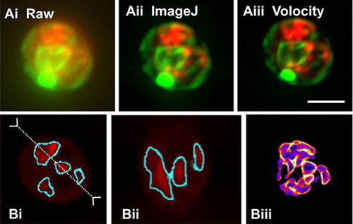
Maximum intensity z-projections of (Ai) the raw data, (Aii) after iterative deconvolution with ImageJ (2 h processing time), and (Aiii) after iterative deconvolution in Volocity (5 min processing time). Scale bar, 2.5 µm. (B) The volume of the mitochondria in the red channel of the Volocity deconvolved data was quantified in ImageJ using the TransfomJ and Object Counter three-dimensional (3-D) plugins. The volume of the mitochondria was calculated as 12.0 µm3 (the volume calculated in Volocity with the same threshold was 12.1 µm3). (Bi) Median section (slice 90) of deconvolved stack overlaid with the object boundaries identified by the ImageJ plugin. (Bii) The axial section along the y-y′ line from BI showing object boundaries in cyan. (Biii) Summed z-projection of the stack of identified object boundaries.
The accessibility of the source code has also made ImageJ a favorite for development and implementation of fluorescence resonance energy transfer (FRET) image analysis. There are various plugins available that perform sensitized emission and acceptor photo-bleaching analysis of FRET image sequences. We are also using ImageJ to analyze lifetime images that have been acquired, processed, and exported from our Becker and Hickl TCSPC system.
Co-Localization Analysis
Another key advantage of ImageJ is its abilities in co-localization analysis. Given that no single co-localization quantification technique is appropriate for all circumstances, ImageJ's large suite of co-localization plugins provides options for this additional functionality. Since users are not restricted to a specific approach, the most appropriate co-localization technique from the toolbox can be chosen. Among others, plugins are available to perform qualitative overlays [and convert them from Red-Green-Blue (RGB) to the color-blind friendly Magenta-Green-Blue], generate Pearson's coefficients, generate Mander's coefficients, and perform various randomization co-localization tests [e.g., Fay (1), Costes (2), and van Steensel (3)]. However, as with all analysis tools, they can be misused, and researchers are encouraged to understand these analyses before selecting and using one. The open-source nature of ImageJ also allows the development of novel co-localization routines. Intensity correlation analysis by Li and colleagues was refined only after implementation in ImageJ enabled an improved rate of analysis (4,5).
Z-Functions
In addition to the standard z-projections and axial sectioning, ImageJ also has some sophisticated three-dimensional (3-D) reconstruction routines. VolumeJ from Michael Abramoff generates ray-traced surface rendering of z-series (Figure 3). This plugin employs a user-defined threshold to generate a surface-rendered image. It can be used to with RGB multichannel or depth-coded images and to generate rotational movies.

Confocal z-series of 40 µM thick 4′,6-diamidino-2-phenylindole (DAPI)-stained mouse aorta showing the nuclei in the different smooth muscle layers. Sample provided by M. Kahn (McMaster University). Scale bars, 30 µm.
T-Functions
One of the quirks of ImageJ is the presumption that a stack's third dimension will be the z-axis. An intensity versus time plot can be performed by the menu command Plot z-axis profile (Figure 4). ImageJ supports a number of time course processing and analysis routines. This includes bleach correction for visualization, normalization to initial intensity, ratio-imaging, and delta-fluorescence routines. The core region of interest (ROI) manager allows multiple regions of interest to be analyzed (and the ROIs saved), greatly facilitating intensity versus time studies, such as calcium imaging. With Rasband's help, we have recently integrated a ratiometric analysis plugin with the ROI manager, again, facilitating analysis, and also providing a plugin template for multi-region processing for other types of analysis.

(A) Median intensity projection of the time-course to illustrate a puffsite (circle) and the axis of the pseudo-linescan plot (x-x′). Scale bar 10, µm. (B) Intensity versus time plot of the puffsite region of interests (ROI; circle in panel A) generated by the Plot z-axis profile menu command. ImageJ assumes the third axis of a stack is z. The raw data was processed for F÷F0 prior to analysis. (C) Intensity versus xt pseudo-linescan image of the line (x-x′) drawn in panel A. Contrast was adjusted to improve visualization of the calcium puffs that precede the global signal. (D) Surface plot of image C using the Interactive three-dimensional (3-D) Surface Plot plugin. (E) Intensity versus xyt. Frames taken from a surface plot movie of the F÷F0 processed image stack generated using the Surface Plot menu command.
Particle Analysis
The integral Particle Analyzer is a powerful multi-region detection and analysis routine. Along with particle separation based on watershed or maxima parameters, ImageJ's core program provides a range of options for users. Plugins add to this functionality with 3-D particle measurements and various particle tracking routines.
Macros and Plugins
The internal macro programming language of ImageJ is a simple text-based scripting language that can be used just to automate multiple processing and analysis steps and batch processing, but can also evolve into very sophisticated routines. First attempts at writing macros are easily undertaken using the macro recorder function to record the menu commands a user wants to automate. This initial macro can then be further developed using the macro programming language, which is well documented on the ImageJ web site.
The ImageJ web site also hosts many sample macros that can be modified to suit specific needs. There are several generic batch-processing macros that will automate a series of commands on all images in a folder or even all images in subfolders.
While macros can become quite sophisticated, the real power of ImageJ is the plugins. As with macros, a user unfamiliar with Java can start by editing the source code of existing plugins.
ImageJ Resources
Once installed, the core ImageJ program (the IJ.JAR file) can be easily upgraded by simply downloading it from the NIH web site. Keeping an eye on the News page on the ImageJ web site provides a quick summary of what's new with core ImageJ functionality and user-written plugins and macros.
The MacBiophotonics ImageJ for Microscopy online manual is a useful resource for new users of ImageJ, covering the typical image processing and analysis steps for microscopists. More complex issues can be addressed via the ImageJ mailing list, an excellent source of information and assistance. The mailing list archives are searchable from the ImageJ web site and usually throw up the answer—many questions have already been addressed. Failing this, a detailed description of the problem to the user group usually results in a quick response with the solution. A recent example of this came when I tried to integrate the ROI manager with a ratio-analysis plugin I had already written. My efforts resulted in a functional, but very slow plugin—taking approximately. I min to analyze a 600-frame stack. A detailed note to the mailing list was met with a quick fix that reduced the analysis to a far more respectable 5 s. This example also addresses one of the perceptions that Java is intrinsically slow. Since Java is highly accessible, functional rather than efficient code can be written by users such as myself with programming-enthusiasm rather than formal training. However, whether a function is executed in 1 or 2 s is probably not relevant except in extreme batch processing of thousands of images.
There is an increasing interest in ImageJ at international meetings and workshops. The first ImageJ user and developer conference was held in 2006, and Microscopy and Microanalysis in 2007 will have a session (Symposium A16) dedicated to ImageJ. A number of ImageJ workshops are also cropping up. An ImageJ lab will form an integral part of our Practical Biophotonics introductory workshop that we are hosting in mid-July 2007 and is planned to be a significant part of one of the advanced workshops in the series (www.macbiophotonics.ca/workshop).
Summary
ImageJ is an essential tool for us that fulfills most of our routine image processing and analysis requirements. The near-comprehensive range of import filters that allow easy access to image and meta-data, a broad suite processing and analysis routine, and enthusiastic support from a friendly mailing list are invaluable for all microscopy labs and facilities—not just those on a budget.
Acknowledgments
I am grateful to Wayne Rasband and the plugin authors who have made their work freely available to the scientific community. MacBiophotonics is supported by the Canadian Foundation for Innovation and the Ontario Innovation Trust.
References
- 1. . 1997. Quantitative digital analysis of diffuse and concentrated nuclear distributions of nascent transcripts, SC35 and poly(A). Exp. Cell Res. 231:27–37.
- 2. . 2004. Automatic and quantitative measurement of protein-protein colocalization in live cells. Biophys. J. 86:3993–4003.
- 3. . 1996. Partial colocalization of glucocorticoid and mineralocorticoid receptors in discrete compartments in nuclei of rat hippocampus neurons. J. Cell Sci. 109:787–792.
- 4. . 2006. N type Ca2+ channels and RIM scaffold protein covary at the presynaptic transmitter release face but are components of independent protein complexes. Neuroscience 140:1201–1208.
- 5. . 2004. A syntaxin 1, Galpha(o), and N-type calcium channel complex at a presynaptic nerve terminal: analysis by quantitative immunocolocalization. J. Neurosci. 24:4070–4081.
- 6. . 1990. Proposed standard for image cytometry data files. Cytometry 11:561–569.


